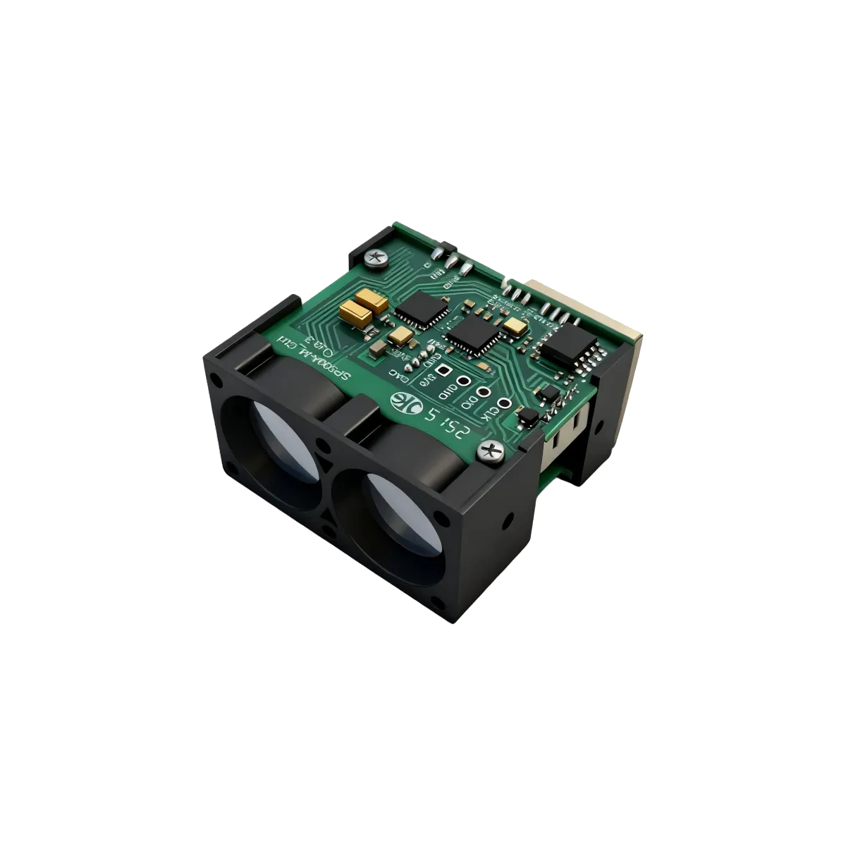
When LRF600H measurement frequency changes, a fixed smoothing coefficient can change the display’s response time even if the filter code stays the same. For an industrial distance display or logger, define smoothing in seconds and calculate the coefficient from trustworthy elapsed time. Keep stale-data handling separate: a smoother cannot recover observations that were never received.
The documented rate change
The current LRF600H documentation specifies a measurement frequency of 1 kHz or 50 Hz, switching automatically to match echo strength. ERDI checked that model-specific entry on 26 September 2026. The corresponding ideal periods are calculated as dt = 1 / f: 0.001 s and 0.020 s. These are nominal calculation inputs, not measured arrival intervals or a maximum communication-delay guarantee.
The existing high-rate integration guide discusses filtering, validity and latency. Here the narrower question is why a display tuned at one rate can feel much slower at another, and how to check that behavior without a physical sensor.
A coefficient remembers samples, not seconds
A simple exponentially weighted moving average uses y_new = y_old + alpha * (x - y_old), where x is the accepted distance, y is the smoothed distance and alpha is a dimensionless weight between zero and one. This is the recurrence described in the NIST EWMA reference, with alpha replacing its symbol lambda. We use only that averaging rule here, not the reference’s statistical control limits or suggested weights.
For a constant input, the remaining error after n updates is error_n = error_0 * (1 - alpha)^n. Equating that decay with exp(-n * dt / tau) gives tau = -dt / ln(1 - alpha). Tau is the calculated time constant: after one tau, about 63.2% of a sustained step has been followed. It is not a sensor response specification.
Assume alpha = 0.1, one valid update per ideal period, no transport delay and an already initialized filter. The weight is an invented host setting. At 1 kHz, tau is about 9.49 ms; at 50 Hz, it is about 189.82 ms. Thus the same coefficient makes this mathematical response twenty times slower in elapsed time. That does not prove a real module’s end-to-end latency changed by the same factor.
Choose a time constant and derive the weight
Rearranging the same decay equation gives alpha = 1 - exp(-dt / tau). As a worked example, choose tau = 0.100 s for a host display. This choice illustrates the arithmetic; it is neither an LRF600H setting nor a recommended control-loop delay.
| Ideal valid-update rate | dt | Calculated alpha | Updates in 100 ms |
|---|---|---|---|
| 1 kHz | 0.001 s | 0.00995017 | 100 |
| 50 Hz | 0.020 s | 0.18126925 | 5 |
Initialize y to a synthetic 4 m at time zero, then supply only synthetic 6 m values. Make the first update after one full period. At 100 ms both sequences give y = 6 + (4 - 6) * exp(-0.100 / 0.100), or about 5.26424 m. A mixed sequence of twenty 1 ms intervals followed by four 20 ms intervals has the same total duration and result. This equivalence holds for the constant input in this exercise; arbitrary moving inputs sampled at different times will not generally produce identical outputs.
In software, alpha = -expm1(-dt / tau) avoids subtracting two nearly equal numbers when dt/tau is small. The official Python math documentation explains this numerical advantage of expm1. Use positive, finite tau and dt, in the same time units.
Make time and missing-data rules explicit
Use the interval between accepted observations from a consistent, monotonic time base. Timestamp reports as close to acquisition as the host permits. Host reception timestamps describe reception, not the instant of optical measurement. If a serial adapter releases many buffered reports together, their callback spacing cannot establish their original sample spacing. Do not reconstruct that spacing by assuming either nominal rate during an unknown transition; flag the timing uncertainty and improve the capture path.
For this display example, reject invalid observations before filtering and do not advance the last-valid timestamp on them. Check an application-defined freshness limit even during silence. If that limit expires, mark the output unavailable. On recovery, initialize from the first fresh valid observation instead of blending across the unknown gap. The freshness limit is an application requirement, not a number established by the frequency row.
For shorter accepted gaps, the elapsed-time rule assigns the new value a larger weight. This is an explicit estimator choice, not evidence that the new distance existed throughout the gap. Preserve the raw values and timestamps so that smoothing does not conceal a real change, sparse observations or transport faults.
Acceptance checks for the host implementation
- Fixed-weight baseline: replay the synthetic step with alpha = 0.1. At 100 ms, expect about 5.99995 m after 100 updates, but 4.81902 m after five. This exposes the sample-count dependency.
- Time-based weight: use tau = 0.100 s and each sequence’s dt. Expect approximately 5.26424 m at 100 ms for both uniform sequences and the mixed sequence above. Use unrounded coefficients internally.
- Bad timestamps: inject equal, decreasing or non-finite timestamps. Reject the affected update, record a timing fault and leave the accepted state unchanged.
- Silence and recovery: advance the test clock past the application’s freshness limit without callbacks. Expect unavailable status; the next fresh valid sample initializes a new filter state.
- Buffered delivery: deliver an old batch together. Confirm that the application exposes uncertain timing rather than reporting a successfully verified measurement cadence.
These are calculated software acceptance cases, not laboratory results. Matching the decay envelope does not restore lost temporal detail, establish optical accuracy or validate a machine safety function. For a documentation check, contact ERDILRF with your model, timestamp method and a short report trace.