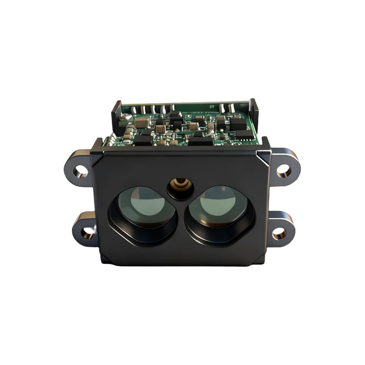
A steady LRF50H distance display does not establish that the distance is correct. During a stationary fixture check, calculate both the average error against an independent reference and the spread of repeated valid readings. A narrow cluster can still sit on the wrong side of the reference. Keep those two results separate before deciding whether to investigate alignment, the reference setup or the sensor.
What the model documentation does, and does not, say
ERDI’s documentation review on 27 September 2026 checked the LRF50H accuracy entry: ±5 cm below 10 m and 1% at or above 10 m, with the stated 2σ qualifier. The repeatability entry is separately listed as ±5 cm. Preserve both entries as written: the repeatability row does not specify a sample count or statistical definition. Do not reinterpret that ±5 cm as a standard deviation, or turn the accuracy entry into a maximum-error promise for every individual reading.
Our existing high-rate integration guide recommends separating offset, repeatability and other error sources. The exercise below makes that distinction calculable for an incoming inspection of a stationary industrial distance logger. It is a diagnostic method, not a factory acceptance rule or a report of measurements performed by ERDILRF.
Two artificial records with the same spread
Assume an ideal reference distance R = 5.00 m, a stationary flat surface and five valid distances per record. All distances below are invented, already decoded values in metres; five is chosen only to make the arithmetic easy to inspect. No output rate, operating mode, target reflectivity or real-device performance is implied. Treating the reference as exact is an arithmetic assumption that must be replaced by a documented reference uncertainty in an actual inspection.
| Quantity | Record A | Record B |
|---|---|---|
| Five distances, m | 4.99, 5.00, 5.01, 5.00, 5.00 | 5.09, 5.10, 5.11, 5.10, 5.10 |
| Mean, m | 5.00 | 5.10 |
| Mean minus reference, m | 0.00 | +0.10 |
| Sample standard deviation, m | 0.00707 | 0.00707 |
For n readings xi, compute the mean x̄ = Σxi / n, the observed mean error b = x̄ − R, and the sample standard deviation s = √[Σ(xi − x̄)² / (n − 1)]. The spread calculation requires n ≥ 2. In both records the deviations from their own mean are −0.01, 0, +0.01, 0 and 0 m. Thus s = √(0.0002 / 4) = 0.007071… m, approximately 0.71 cm.
Adding 0.10 m to every entry moves the mean without changing that spread. Record B therefore looks just as steady as A, while its observed mean error is 10 cm. Averaging more readings would not remove an unchanged additive offset. These short records illustrate a distinction; they do not estimate long-term performance or establish that a unit passes or fails its documented specification.
The NIST discussion of bias and accuracy relates bias to the difference between a measurement average and a reference value. Here b is a finite-record estimate relative to the chosen reference, not proof of the sensor’s intrinsic bias. NIST’s separate discussion of variability uses standard deviation to describe short-term precision and cautions that variation over longer periods can be larger.
A fixture check that preserves the evidence
- Define the distance being compared. Record the sensor’s measurement datum, the reference instrument’s datum and the same surface point along the intended measurement direction. If the module datum is unclear, obtain its definition before attributing a constant difference to the sensor. A housing edge and an optical reference plane are not automatically interchangeable.
- Freeze the setup. Record model, unit identifier, document revision, firmware if available, output configuration, fixture position, surface material, incidence angle, illumination, temperature and window condition. State the reference method and its uncertainty. Do not infer numerical reflectivity from a surface’s colour.
- Save the unfiltered record. Keep timestamps and validity information. Count invalid reports separately, following the existing LRF50H invalid-value handling example. Do not replace missing observations with zero or repeat the last distance. Report the acquisition duration and valid count alongside the statistics.
- Calculate before correcting. Save R, n, x̄, b and s for each stationary position. Never compute spread around the reference and label it repeatability: that mixes offset into the spread. A smooth display produced by host filtering is also a different record from the raw readings.
- Investigate the pattern. Small spread with a persistent mean difference calls for checking the reference, datum and geometry first. Large spread calls for examining surface stability, mount movement and changing optical conditions. These are investigation paths, not diagnoses proved by either statistic.
- Check another position and a fresh run. Keep position-specific results separate. A similar offset at two positions suggests a different follow-up from an error that grows with distance, but neither pattern proves its cause. Any proposed correction must be evaluated on new observations and relevant operating conditions, not only on the record used to choose it.
Set inspection limits and the sampling plan before collecting production evidence. Include reference uncertainty, relevant conditions and an agreed interpretation of the specification’s 2σ qualifier; this note supplies no replacement pass threshold. Closely spaced readings may be correlated, so the number of logged reports alone does not establish the uncertainty of the mean. If the reference uncertainty or measurement datum is unknown, retain the result as a diagnostic observation and leave conformance undecided.
For help reconciling a fixture check with the documentation, contact ERDILRF with the model, reference method, setup sketch and a short unfiltered record.